Particle Filtering
Matthieu Bloch
Tuesday, November 8, 2022
Today in ECE 6555
- Announcements
- 8 lectures left (including today)
- Kalman filtering mini project due November 10, 2022
- Last time
- Extended Kalman Filter (EKF) from Bayesian filtering
- Introduction to Unscented Kalman Filter (UKF)
- Today
- Particle Filtering
- Questions?
Last Time: Extended Kalman filter revisited
- The Kalman filter is an approximate Bayesian optimal filter
- Initialization: \(x_0\sim\calN(\hat{x}_{0|-1},P_0)\)
- Prediction: \(x_{i|i-1}\sim\calN(\hat{x}_{i|i-1},P_{i|i-1})\) with
- Update: \(x_{i|i}\sim\calN(\hat{x}_{i|i},P_{i|i})\) with
\[ \begin{aligned} \hat{x}_{i|i} &= \hat{x}_{i|i-1}+K_{f,i}(y_i-h(\hat{x}_{i|i-1}))\\ K_{f,i} &= P_{i|i-1}H_x(\hat{x}_{i-1|i-1})^\intercal(H_x(\hat{x}_{i-1|i-1})P_{i|i-1}H_x(\hat{x}_{i-1|i-1})^\intercal+R_i)^{-1}\\ P_{i|i}&= P_{i|i-1}-K_{f,i}H_x(\hat{x}_{i-1|i-1}) P_{i|i-1} \end{aligned} \]
Last Time: Wrapping up EKF
EKF is based on Taylor series expansions of \(f\) and \(h\) around current state estimate
Advantages of EKF
- Almost same as basic Kalman filter, easy to use
- Intuitive, engineering way of constructing approximations
- Works very well in practical estimation problems.
- Computationally efficient
Limitations of EKF
- Does not work with strong non-linearities
- Only Gaussian noise processes are allowed
- Measurement model and dynamic model functions need to be differentiable
- Computation and programming of Jacobian matrices can be quite error prone
Linearization assumes that all second and higher order terms in Taylor series expansion are negligible
- In some situations, higher order terms have negligible effects
- In others, they can significantly degrade estimator performance.
Possible to extend EKF approach to higher order terms
- Second-order Gaussian filter
- Assumes piece-wise quadratic model and truncates Taylor series expansion after second term
- Hessian required
Last Time: Unscented Kalman Filter
- Need for a method that is:
- Provably more accurate than linearization;
- Does not incur computational costs of other higher order filtering schemes
- Key observation: Easier to approximate a pdf than an arbitrary nonlinear transformation
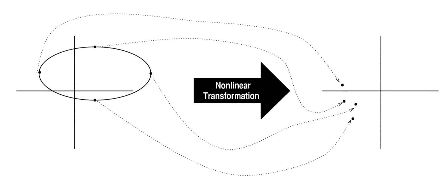
- Unscented transform
- Choose a set of points (sigma points)
- Nonlinear function is applied to each point to yield a cloud of transformed points
- Statistics of transformed points calculated to form estimate of nonlinearly transformed mean and covariance
Unscented Kalman Filter
- Key features
- Sigma points are not drawn at random
- High-order information about the distribution captured with a fixed small number of points
- Sigma points can be weighted in ways that are inconsistent with the distribution interpretation of sample points in a particle filter.
- General Sigma-point selection
framework
- No practical filter can maintain the full distribution of the state
- Simpler distribution of the form may be heuristically assumed, e.g., Gaussian
- Goal is to match different properties of a given distribution, e.g., moments
- In general, find sigma points \(\calS\) that solve
Unscented Kalman Filter
Matching mean and covariance of a Gaussian \[ \begin{aligned} \mathbf{c}_1[\calS,p_x(\bfx)]&=\sum_{i=0}^p w^{(i)}\bfx^{(i)} - \bar{\bfx}\\ \mathbf{c}_2[\calS,p_x(\bfx)]&=\sum_{i=0}^p w^{(i)}(\bfx^{(i)}-\bar{\bfx})(\bfx^{(i)}-\bar{\bfx})^\intercal - \Sigma_x\\ \end{aligned} \]
Solution: set of points that lie on the \(\sqrt{N_x}\) covariance contour
- \(p = 2N_x\), \(w^{(0)}=0\)
- For \(i\in\intseq{1}{N_x}\) \(\bfx^{(i)}= \bar{\bfx}+(\sqrt{N_x\Sigma_x})_i\) and \(w^{(i)} = \frac{1}{2N_x}\)
- For \(i\in\intseq{N_x+1}{2N_x}\) \(\bfx^{(i)}= \bar{\bfx}-(\sqrt{N_x\Sigma_x})_i\) and \(w^{(i)} = \frac{1}{2N_x}\)
- \(\Sigma_x = \sqrt{\Sigma_x}\sqrt{\Sigma_x}^\intercal\) with \((\sqrt{\Sigma_x})_i\) \(i\)-th column
Propagate sigma points through non-linear transform
- \(\bar{\bfy} = \sum_{i}w^{(i)}h(\bfx^{(i)})\)
- \(\sum_{i} w^{(i)}(h(\bfx^{(i)})-\bar{\bfy})(h(\bfx^{(i)})-\bar{\bfy})^\intercal\)
Monte-Carlo approximations
- Gaussian approximation often work well…
- but cannot capture multi-modal distributions, discrete components, etc.
- Particle filters are Monte-Carlo methods to approximate the solution of Bayesian Filtering
- Monte Carlo approximation
- The central difficulty in Bayesian inference is to compute \[ \E{g(\vecx)|\vecy_{1:T}} \eqdef \int g(\vecx)p(\vecx|\vecy_{1:T})d\vecx \] where \(g:\bbR^n\to\bbR^m\)
- No closed-form expression in general
- Approach
- Draw \(n\) samples \(\vecx_i\sim p(\vecx|\vecy_{1:T})\)
- Estimate \[ \E{g(\vecx)|\vecy_{1:T}} \approx \frac{1}{n}\sum_{i=1}^n g(\vecx_i) \]
- Converge in \(\calO(n^{-1/2})\) regardless of dimension
Importance sampling
- It might still be challenging to sample according to \(p(\vecx|\vecy_{1:T})\) (complicated functional form)
- Importance sampling
- Use an importance distribution \(\pi(\vecx|\vecy_{1:T})\) \[ \E{g(\vecx)|\vecy_{1:T}} \eqdef \int g(\vecx)p(\vecx|\vecy_{1:T})d\vecx = \int g(\vecx)\frac{p(\vecx|\vecy_{1:T})}{\pi(\vecx|\vecy_{1:T})}\pi(\vecx|\vecy_{1:T})d\vecx \] assuming \(\pi(\vecx|\vecy_{1:T}) \ll p(\vecx|\vecy_{1:T})\)
- Draw \(n\) samples \(\vecx^{(i)}\sim \pi(\vecx|\vecy_{1:T})\)
- Estimate \[ \E{g(\vecx)|\vecy_{1:T}} \approx \sum_{i=1}^n \tilde{w}^{(i)} g(\vecx^{(i)})\textsf{ where } \tilde{w}^{(i)} \eqdef \frac{1}{n}\frac{p(\vecx^{(i)}|\vecy_{1:T})}{\pi(\vecx^{(i)}|\vecy_{1:T})} \]
- Challenge: assumes that we can evaluate \(p(\vecx^{(i)}|\vecy_{1:T})\)
Importance sampling
In general, \(p(y_{1:T}|\vecx^{(i)})\) easier to evaluate (measurement model)
Use Bayes' rule \[ p(\vecx^{(i)}|\vecy_{1:T}) = \frac{p(y_{1:T}|\vecx^{(i)})p(\vecx^{(i)})}{\int p(y_{1:T}|\vecx)p(\vecx)d\vecx} \] and note the denominator is still hard to compute!
Importance sampling to the rescue \[ \E{g(\vecx)|\vecy_{1:T}} \approx \sum_{i=1}^n \tilde{w}^{(i)} g(\vecx^{(i)})\textsf{ where } \tilde{w}^{(i)} \eqdef \frac{\frac{p(\vecy_{1:T}|\vecx^{(i)})p(\vecx^{(i)})}{\pi(\vecx^{(i)}|\vecy_{1:T})}}{\sum_{j=1}^n\frac{p(\vecy_{1:T}|\vecx_j)p(\vecx_j)}{\pi(\vecx_j|\vecy_{1:T})}} \]
Importance sampling algorithm
- Assume measurement model \(p(\vecy_{1:T}|\vecx)\) and prior \(p(\vecx)\)
- Draw \(n\) samples \[ \vecx^{(i)}\sim \pi(\vecx|\vecy_{1:T})\quad i=1\dots n \]
- Compute unnormalized weights \[ v^{(i)} = \frac{p(\vecy_{1:T}|\vecx^{(i)})p(\vecx^{(i)})}{\pi(\vecx^{(i)}|\vecy_{1:T})} \]
- Compute normalized weights \[ w^{(i)} = \frac{v^{(i)}}{\sum_{j=1}^n v_j} \]
- Approximate posteriors \[ p(\vecx|\vecy_{1:T})\approx \sum_{i=1}^n w^{(i)}\delta(\vecx-\vecx^{(i)})\qquad \E{g(\vecx)|\vecy_{1:T}}\approx \sum_{i=1}^n w^{(i)} g(\vecx^{(i)}) \]
Sequential importance sampling
Sequential importance sampling is a variation that can be used for probabilistic state-space models with \[ \vecx_k\sim p(\vecx_k|\vecx_{k-1})\qquad \vecy_k\sim p(\vecy_k|\vecx_k) \]
Idea
- Keep track of particles \(\set{(w^{(i)}_{k},\vecx^{(i)}_k):i=1\dots n}\) at every time \(k\) to compute \[ p(\vecx_k|\vecy_{1:k})\approx \sum_{i=1}^n w_k^{(i)}\delta(\vecx_k-\vecx_k^{(i)})\qquad \E{g(\vecx_k)|\vecy_{1:k}}\approx \sum_{i=1}^n w_k^{(i)} g(\vecx_k^{(i)}) \]
- Use properties of state-space model to only keep track of current states at time \(k\), not entire history
Sequential importance sampling
- Draw \(n\) samples from the prior \[ \vecx_0^{(i)}\sim p(\vecx_0)\quad i=1\dots n \] and set \(w^{(i)}=\frac{1}{n}\) for \(i=1\dots n\)
- For each \(k=1\dots T\)
- Draw samples \(\vecx_k^{(i)}\) from importance distributions \[ \vecx_k^{(i)}\sim \pi(\vecx_k|\vecx^{(i)}_{0:k-1}\vecy_{1:k})\quad i=1\dots n \]
- Compute new weights \[ w_k^{(i)}\propto w_{k-1}^{(i)} \frac{p(\vecy_k|\vecx_k^{(i)})p(\vecx_k^{(i)}|\vecx_{k-1}^{(i)})}{\pi(\vecx_k^{(i)}|\vecx_{0:k-1}^{(i)},\vecy_{1:k})} \] and normalize
- Try to choose \(\pi(\vecx_k|\vecx_{0:k-1},\vecy_{1:k})=\pi(\vecx_k|\vecx_{k-1},\vecy_{1:k})\)
Particle filter
- Resampling might be needed when weights get too low (particles disappear)
- Draw \(n\) samples from the prior \(\vecx_0^{(i)}\sim p(\vecx_0)\quad i=1\dots n\) and set \(w^{(i)}=\frac{1}{n}\) for \(i=1\dots n\)
- For each \(k=1\dots T\)
- Draw samples \(\vecx_k^{(i)}\) from importance distributions \[ \vecx_k^{(i)}\sim \pi(\vecx_k|\vecx^{(i)}_{0:k-1}\vecy_{1:k})\quad i=1\dots n \]
- Compute new weights \[ w_k^{(i)}\propto w_{k-1}^{(i)} \frac{p(\vecy_k|\vecx_k^{(i)})p(\vecx_k^{(i)}|\vecx_{k-1}^{(i)})}{\pi(\vecx_k^{(i)}|\vecx_{0:k-1}^{(i)},\vecy_{1:k})} \] and normalize
- If effective number of particles get too low, resample and reset to uniform weights \[ n_\textsf{eff}\approx\frac{1}{\sum_{j=1}^n (w_k^{(i)})^2} \]