Learning

Logistics

• General announcements

  • Assignment 6 posted (last assignment)

  • Due December 7, 2021 for bonus, deadline December 10, 2021

  • 2 lectures left

  • Let me know what’s missing

• Assignment 5 grades posted

• Reviewing Midterm2 grades one last time

What’s on the agenda for today?

• The learning problem and why we need probabilities.

• Lecture notes 17 and 23

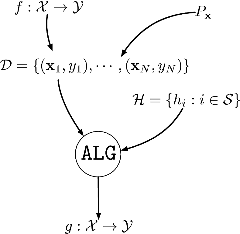
Components of supervised machine learning

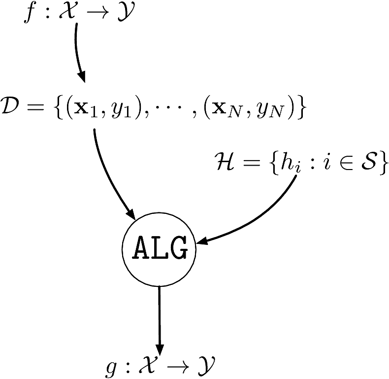
1. An unknown function \(f:\calX\to\calY:\bfx\mapsto y=f(\bfx)\) to learn
   • The formula to distinguish cats from dogs
2. A dataset \(\calD\eqdef\{(\bfx_1,y_1),\cdots,(\bfx_N,y_N)\}\)
   • \(\bfx_i\in\calX\eqdef\bbR^d\): picture of cat/dog
   • \(y_i\in\calY\eqdef\bbR\): the corresponding label cat/dog
3. A set of hypotheses \(\calH\) as to what the function could be
   • Example: deep neural nets with AlexNet architecture
4. An algorithm \(\texttt{ALG}\) to find the best \(h\in\calH\) that explains \(f\)

• Terminology:
  • \(\calY=\bbR\): regression problem
  • \(\card{\calY}<\infty\): classification problem
  • \(\card{\calY}=2\): binary classification problem
• The goal is to generalize, i.e., be able to classify inputs we have not seen.

A learning puzzle

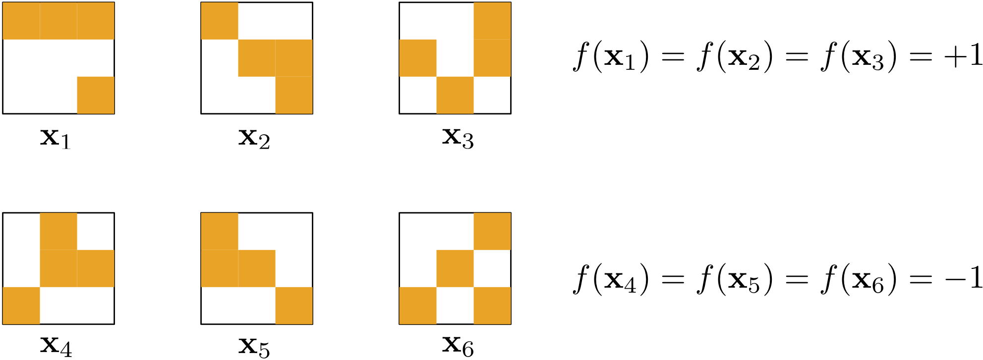
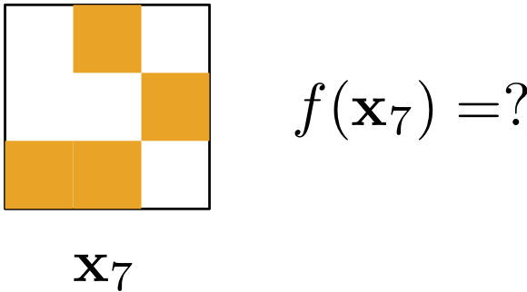
• Learning seems impossible without additional assumptions!

Possible vs probable

• Flip a biased coin, lands on head with unknown probability \(p\in[0,1]\)

• \(\P{\text{head}}=p\) and \(\P{\text{tail}}=1-p\)

• Say we flip the coin \(N\) times, can we estimate \(p\)?

• \[ \hat{p} = \frac{\text{\# head}}{N} \]

• Can we relate \(\hat{p}\) to \(p\)?

  • The law of large numbers tells us that \(\hat{p}\) converges in probability to \(p\) as \(N\) gets large \[ \forall\epsilon>0\quad\P{\abs{\hat{p}-p}>\epsilon}\mathop{\longrightarrow}_{N\to\infty} 0. \]

• It is possible that \(\hat{p}\) is completely off but it is not probable

Components of supervised machine learning

1. An unknown function \(f:\calX\to\calY:\bfx\mapsto y=f(\bfx)\) to learn

2. A dataset \(\calD\eqdef\{(\bfx_1,y_1),\cdots,(\bfx_N,y_N)\}\)

   • \(\{\bfx_i\}_{i=1}^N\) i.i.d. from unknown distribution \(P_{\bfx}\) on \(\calX\)
   • \(\{y_i\}_{i=1}^N\) are the corresponding labels \(y_i\in\calY\eqdef\bbR\)

3. A set of hypotheses \(\calH\) as to what the function could be

4. An algorithm \(\texttt{ALG}\) to find the best \(h\in\calH\) that explains \(f\)

Another learning puzzle

Components of supervised machine learning

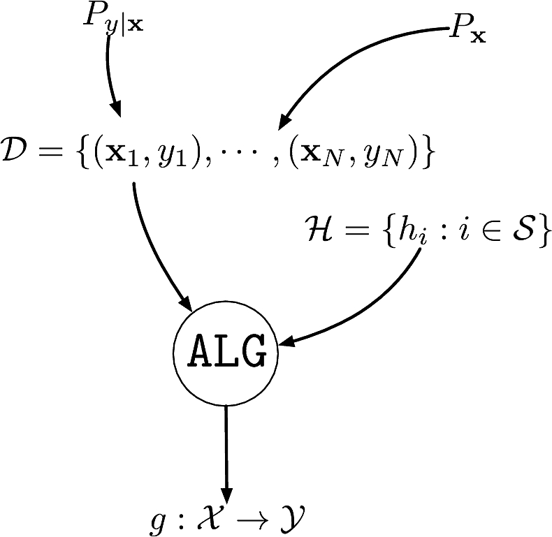
1. An unknown conditional distribution \(P_{y|\bfx}\) to learn

   • \(P_{y|\bfx}\) models \(f:\calX\to\calY\) with noise

2. A dataset \(\calD\eqdef\{(\bfx_1,y_1),\cdots,(\bfx_N,y_N)\}\)

   • \(\{\bfx_i\}_{i=1}^N\) i.i.d. from distribution \(P_{\bfx}\) on \(\calX\)
   • \(\{y_i\}_{i=1}^N\) are the corresponding labels \(y_i\sim P_{y|\bfx=\bfx_i}\)

3. A set of hypotheses \(\calH\) as to what the function could be

4. An algorithm \(\texttt{ALG}\) to find the best \(h\in\calH\) that explains \(f\)

• The roles of \(P_{y|\bfx}\) and \(P_{\bfx}\) are different
  • \(P_{y|\bfx}\) is what we want to learn, captures the underlying function and the noise added to it
  • \(P_{\bfx}\) models sampling of dataset, need not be learned

Yet another learning puzzle

• Assume that you are designing a fingerprint authentication system
  • You trained your system with a fancy machine learning system
  • The probability of wrongly authenticating is 1%
  • The probability of correctly authenticating is 60%
  • Is this a good system?
• It depends!
  • If you are GTRI, this might be ok (security matters more)
  • If you are Apple, this is not acceptable (convenience matters more)
• There is an application dependent cost that can affect the design

Components of supervised machine learning

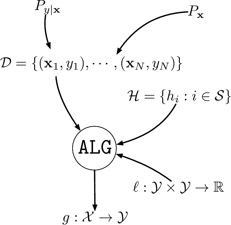
1. A dataset \(\calD\eqdef\{(\bfx_1,y_1),\cdots,(\bfx_N,y_N)\}\)

   • \(\{\bfx_i\}_{i=1}^N\) i.i.d. from an unknown distribution \(P_{\bfx}\) on \(\calX\)

2. An unknown conditional distribution \(P_{y|\bfx}\)

   • \(P_{y|\bfx}\) models \(f:\calX\to\calY\) with noise
   • \(\{y_i\}_{i=1}^N\) are the corresponding labels \(y_i\sim P_{y|\bfx=\bfx_i}\)

3. A set of hypotheses \(\calH\) as to what the function could be

4. A loss function \(\ell:\calY\times\calY\rightarrow\bbR^+\) capturing the “cost” of prediction

5. An algorithm \(\texttt{ALG}\) to find the best \(h\in\calH\) that explains \(f\)

The supervised learning problem

• Learning is not memorizing

  • Our goal is not to find \(h\in\calH\) that accurately assigns values to elements of \(\calD\)
  • Our goal is to find the best \(h\in\calH\) that accurately predicts values of unseen samples

• Consider hypothesis \(h\in\calH\). We can easily compute the empirical risk (a.k.a. in-sample error) \[\widehat{R}_N(h)\eqdef\frac{1}{N}\sum_{i=1}^N\ell(y_i,h(\bfx_i))\]

• What we really care about is the true risk (a.k.a. out-sample error) \(R(h)\eqdef\E[\bfx y]{\ell(y,h(\bfx))}\)

• Question #1: Can we generalize?

  • For a given \(h\), is \(\widehat{R}_N(h)\) close to \({R}(h)\)?

• Question #2: Can we learn well?

  • The best hypothesis is \(h^{\sharp}\eqdef\argmin_{h\in\calH}R(h)\) but we can only find \(h^{*}\eqdef\argmin_{h\in\calH}\widehat{R}_N(h)\)
  • Is \(\widehat{R}_N(h^*)\) close to \(R(h^{\sharp})\)?
  • Is \(R(h^{\sharp})\approx 0\)?

A simpler supervised learning problem

Consider a special case of the general supervised learning problem

1. Dataset \(\calD\eqdef\{(\bfx_1,y_1),\cdots,(\bfx_N,y_N)\}\)

   • \(\{\bfx_i\}_{i=1}^N\) drawn i.i.d. from unknown \(P_{\bfx}\) on \(\calX\)
   • \(\{y_i\}_{i=1}^N\) labels with \(\calY=\{0,1\}\) (binary classification)

2. Unknown \(f:\calX\to\calY\), no noise.

3. Finite set of hypotheses \(\calH\), \(\card{\calH}=M<\infty\)

   • \(\calH\eqdef\{h_i\}_{i=1}^M\)

4. Binary loss function \(\ell:\calY\times\calY\rightarrow\bbR^+:(y_1,y_2)\mapsto \indic{y_1\neq y_2}\)

• In this very specific case, the true risk simplifies \[ R(h)\eqdef\E[\bfx y]{\indic{h(\bfx)\neq y}} = \P[\bfx y]{h(\bfx)\neq y} \]

• The empirical risk becomes \[ \widehat{R}_N(h)=\frac{1}{N}\sum_{i=1}^{N} \indic{h(\bfx_i)\neq y_i} \]

Can we learn?

• Our objective is to find a hypothesis \(h^*=\argmin_{h\in\calH}\widehat{R}_N(h)\) that ensures a small risk

• For a fixed \(h_j\in\calH\), how does \(\widehat{R}_N(h_j)\) compares to \({R}(h_j)\)?

• Observe that for \(h_j\in\calH\)

  • The empirical risk is a sum of iid random variables \[ \widehat{R}_N(h_j)=\frac{1}{N}\sum_{i=1}^{N} \indic{h_j(\bfx_i)\neq y_i} \]

  • \(\E{\widehat{R}_N(h_j)} = R(h_j)\)

• \(\P{\abs{\widehat{R}_N(h_j)-{R}(h_j)}>\epsilon}\) is a statement about the deviation of a normalized sum of iid random variables from its mean

• We’re in luck! Such bounds, a.k.a, known as concentration inequalities, are a well studied subject

Concentration inequalities: basics

• Let \(X\) be a non-negative real-valued random variable. Then for all \(t>0\) \[\P{X\geq t}\leq \frac{\E{X}}{t}.\]

• Let \(X\) be a real-valued random variable. Then for all \(t>0\) \[\P{\abs{X-\E{X}}\geq t}\leq \frac{\Var{X}}{t^2}.\]

• Let \(\{X_i\}_{i=1}^N\) be i.i.d. real-valued random variables with finite mean \(\mu\) and finite variance \(\sigma^2\). Then \[\P{\abs{\frac{1}{N}\sum_{i=1}^N X_i-\mu}\geq\epsilon}\leq\frac{\sigma^2}{N\epsilon^2}\qquad\lim_{N\to\infty}\P{\abs{\frac{1}{N}\sum_{i=1}^N X_i-\mu}\geq \epsilon}=0.\]

Back to learning

• By the law of large number, we know that \[ \forall\epsilon>0\quad\P[\{(\bfx_i,y_i)\}]{\abs{\widehat{R}_N(h_j)-{R}(h_j)}\geq\epsilon}\leq \frac{\Var{\indic{h_j(\bfx_1)\neq y_1}}}{N\epsilon^2}\leq \frac{1}{N\epsilon^2}\]

• Given enough data, we can generalize

• How much data? \(N=\frac{1}{\delta\epsilon^2}\) to ensure \(\P{\abs{\widehat{R}_N(h_j)-{R}(h_j)}\geq\epsilon}\leq \delta\).

• That’s not quite enough! We care about \(\widehat{R}_N(h^*)\) where \(h^*=\argmin_{h\in\calH}\widehat{R}_N(h)\)

  • If \(M=\card{\calH}\) is large we should expect the existence of \(h_k\in\calH\) such that \(\widehat{R}_N(h_k)\ll R(h_k)\)

• \[ \P{\abs{\widehat{R}_N(h^*)-{R}(h^*)}\geq\epsilon} \leq \P{\exists j:\abs{\widehat{R}_N(h_j)-{R}(h_j)}\geq\epsilon} \]

• \[ \P{\abs{\widehat{R}_N(h^*)-{R}(h^*)}\geq\epsilon} \leq \frac{M}{N\epsilon^2} \]

• If we choose \(N\geq\lceil\frac{M}{\delta\epsilon^2}\rceil\) we can ensure \(\P{\abs{\widehat{R}_N(h^*)-{R}(h^*)}\geq\epsilon}\leq \delta\).

  • That’s a lot of samples!

Concentration inequalities: not so basic

• We can obtain much better bounds than with Chebyshev

• Let \(\{X_i\}_{i=1}^N\) be i.i.d. real-valued zero-mean random variables such that \(X_i\in[a_i;b_i]\) with \(a_i<b_i\). Then for all \(\epsilon>0\) \[\P{\abs{\frac{1}{N}\sum_{i=1}^N X_i}\geq\epsilon}\leq 2\exp\left(-\frac{2N^2\epsilon^2}{\sum_{i=1}^N(b_i-a_i)^2}\right).\]

• In our learning problem \[ \forall\epsilon>0\quad\P{\abs{\widehat{R}_N(h_j)-{R}(h_j)}\geq\epsilon}\leq 2\exp(-2N\epsilon^2)\]

• \[ \forall\epsilon>0\quad\P{\abs{\widehat{R}_N(h^*)-{R}(h^*)}\geq\epsilon}\leq 2M\exp(-2N\epsilon^2)\]

• We can now choose \(N\geq \lceil\frac{1}{2\epsilon^2}\left(\ln \frac{2M}{\delta}\right)\rceil\)

• \(M\) can be quite large (almost exponential in \(N\)) and, with enough data, we can generalize \(h^*\).

• How about learning \(h^{\sharp}\eqdef\argmin_{h\in\calH}R(h)\)?

Learning can work!

• If \(\forall j\in\calH\,\abs{\widehat{R}_N(h_j)-{R}(h_j)}\leq\epsilon\) then \(\abs{R(h^*)-{R}(h^\sharp)}\leq 2\epsilon\).

• How do we make \(R(h^\sharp)\) small?

  • Need bigger hypothesis class \(\calH\)! (could we take \(M\to\infty\)?)
  • Fundamental trade-off of learning

Probably Approximately Correct Learnability

• A hypothesis set \(\calH\) is (agnostic) PAC learnable if there exists a function \(N_\calH:]0;1[^2\to\bbN\) and a learning algorithm such that:

  • for very \(\epsilon,\delta\in]0;1[\),
  • for every \(P_\bfx\), \(P_{y|\bfx}\),
  • when running the algorithm on at least \(N_\calH(\epsilon,\delta)\) i.i.d. examples, the algorithm returns a hypothesis \(h\in\calH\) such that \[\P[\bfx y]{\abs{{R}(h)-R(h^\sharp)}\leq\epsilon}\geq 1-\delta\]

• The function \(N_{\calH}(\epsilon,\delta)\) is called sample complexity

• We have effectively already proved the following result

• A finite hypothesis set \(\calH\) is PAC learnable with the Empirical Risk Minimization algorithm and with sample complexity \[N_\calH(\epsilon,\delta)={\lceil{\frac{2\ln(2\card{\calH}/\delta)}{\epsilon^2}}\rceil}\]

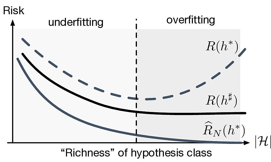
What is a good hypothesis set?

• Ideally we want \(\card{\calH}\) small so that \(R(h^*)\approx R(h^\sharp)\) and get lucky so that \(R(h^*)\approx 0\)

• In general this is not possible

• Remember, we usually have to learn \(P_{y|\bfx}\), not a function \(f\)

• Questions

  • What is the optimal binary classification hypothesis class?
  • How small can \(R(h^*)\) be?