Introduction to VC dimension

Matthieu R Bloch

RECAP: The learning problem

  1. Dataset \(\calD\eqdef\{(\bfx_1,y_1),\cdots,(\bfx_N,y_N)\}\)
    • \(\{\bfx_i\}_{i=1}^N\) drawn i.i.d. from unknown \(P_{\bfx}\) on \(\calX\)
    • \(\{y_i\}_{i=1}^N\) labels with \(\calY=\{0,1\}\) (binary classification)
  2. Unknown \(f:\calX\to\calY\), no noise.

  3. Finite set of hypotheses \(\calH\), \(\card{\calH}=M<\infty\)

    • \(\calH\eqdef\{h_j\}_{j=1}^M\)
  4. Binary loss function \(\ell:\calY\times\calY\rightarrow\bbR^+:(y_1,y_2)\mapsto \indic{y_1\neq y_2}\)

  • True risk and empirical risk: \[ R(h)\eqdef\P[\bfx y]{h(\bfx)\neq y}\qquad \widehat{R}_N(h)=\frac{1}{N}\sum_{i=1}^{N} \indic{h(\bfx_i)\neq y} \]

  • We want to understand when \(\widehat{R}_N(h^*)\approx R(h^*)\) where \(h^*=\argmin_{h\in\calH}\widehat{R}_N(h)\)

Generalization bounds

  • For a hypothesis set \(\calH\) with \(\card{\calH}=M\) we showed that \[ \forall\epsilon>0\quad\P{\abs{\widehat{R}_N(h^*)-{R}(h^*)}\geq\epsilon}\leq 2M\exp(-2N\epsilon^2)\]

  • We used the union bound to introduced the factor \(M\); for any \(\epsilon>0\) \[\P{\abs{\widehat{R}_N(h^*)-{R}(h^*)}\geq\epsilon}\leq \P{\max_{h\in\calH}\abs{\widehat{R}_N(h)-{R}(h)}\geq\epsilon} \leq \sum_{j=1}^M\P{\abs{\widehat{R}_N(h_j)-{R}(h_j)}\geq\epsilon}\]

  • The second inequality is tight if the events \(\calE_j\eqdef \{\abs{\widehat{R}_N(h_j)-{R}(h_j)}\geq\epsilon\}\) are disjoint

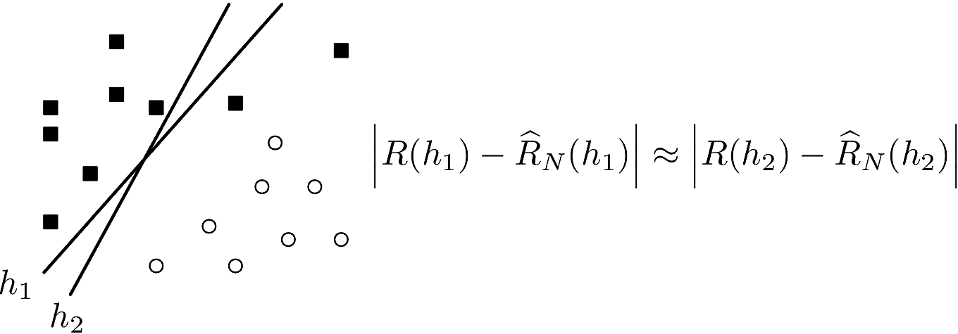
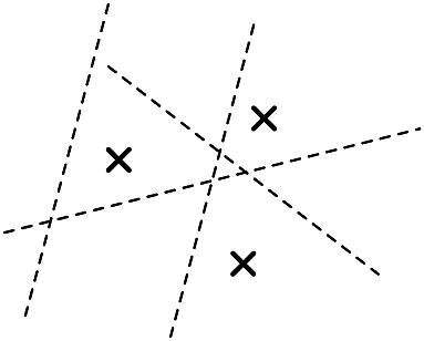
  • Events are not at all disjoint when classifying

Image

Dichotomy

  • The union bound naturally depends on the size of \(\calH\), but this is not what matters

  • We will consider the number of hypotheses that lead to distinct labeling for a dataset

  • For a dataset \(\calD\eqdef \{\bfx_i\}_{i=1}^N\) and set of hypotheses \(\calH\), the set of dichotomies generated by \(\calH\) on \(\calD\) is \[\calH(\{\bfx_i\}_{i=1}^N)\eqdef \{\{h(\bfx_i)\}_{i=1}^N:h\in\calH\}\]

  • By definition \(\card{\calH(\{\bfx_i\}_{i=1}^N)}\leq 2^N\) and in general \(\card{\calH(\{\bfx_i\}_{i=1}^N)}\ll\card{\calH}\)

  • For a set of hypotheses \(\calH\), the growth function of \(\calH\) is \[m_\calH(N)\eqdef\max_{\{\bfx_i\}_{i=1}^N}\card{\calH(\{\bfx_i\}_{i=1}^N)}\]

  • The growth function does not depend on the datapoints \(\{\bfx_i\}_{i=1}^N\) and \(m_{\calH}(N)\leq 2^N\)

Examples

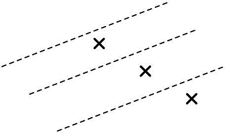
  • Positive rays: \(\calH\eqdef\{h:\bbR\to\{\pm 1\}:x\mapsto \sgn{x-a}| a\in\bbR\}\)
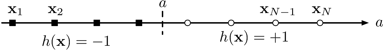
Image
  • \[m_\calH = N+1\]

  • Positive intervals: \(\calH\eqdef\{h:\bbR\to\{\pm 1\}:x\mapsto \indic{x\in[a;b]}-\indic{x\notin[a;b]}| a<b\in\bbR\}\)

Image
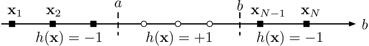
  • \[m_\calH = {N+1 \choose 2}+1 = \frac{1}{2}N^2+\frac{1}{2}N+1\]

Examples

  • Convex sets: \(\calH\eqdef\{h:\bbR^2\to\{\pm 1\}| \{\bfx\in\bbR^2:h(\bfx)=+1\}\textsf{ is convex}\}\)
Image
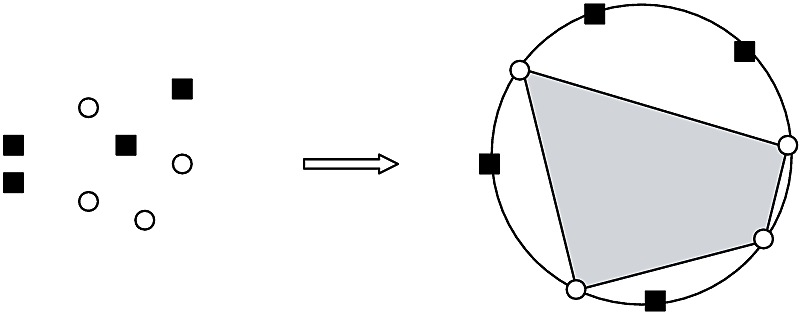
  • \(m_\calH(N)=2^N\) because we can generate all dichotomies

  • If \(\calH\) can generate all dichotomies on \(\{\bfx_i\}_{i=1}^N\), we say that \(\calH\) shatters \(\{\bfx_i\}_{i=1}^N\)

Examples

  • Linear classifiers: \(\calH\eqdef\{h:\bbR^2\to\{\pm 1\}:\bfx\mapsto\sgn{\bfw^\intercal\bfx+b}| \bfw\in\bbR^2,b\in\bbR\}\)
Image
Image
  • The growth function is a worst case measure, hence \(m_{\calH}(3)=8\)
Image
  • 4 points cannot always be shattered and \(m_{\calH}(4)=14<2^4\)

Wishful thinking

  • The growth function \(m_\calH\) can sometimes be smaller than \(\card{\calH}\)

  • What if we could use \(m_\calH\) instead of \(\card{\calH}\) in our analysis?

  • We know that with probability at least \(1-\delta\) \[{R}(h^*)\leq \widehat{R}_N(h^*) +\sqrt{\frac{1}{2N}\log\frac{2\card{\calH}}{\delta}}\]

  • What if we could show that with probability at least \(1-\delta\) \[{R}(h^*)\leq \widehat{R}_N(h^*) +\sqrt{\frac{1}{2N}\log\frac{2m_\calH(N) }{\delta}} \qquad?\]

  • Our ability to generalize then depend on the behavior of the growth function
    • If \(m_{\calH}(N)\) is exponential in \(N\), we can’t say much
    • If \(m_{\calH}(N)\) is polynomial in \(N\), then \({R}(h^*)\approx \widehat{R}_N(h^*)\) for large enough \(N\)

Break points

  • If not data set of size \(k\) can be shattered by \(\calH\), then \(k\) is a break point for \(\calH\)

  • If \(k\) is a break point then \(m_\calH(k)<2^k\)

  • Examples
    • Positive rays: break point \(k=2\)
    • Postive Intervals: break point \(k=3\)
    • Convex sets: break point \(k=\infty\)
    • Linear classifiers: break point \(k=4\)
  • We will spend some time proving the following result

  • If there exists any break point for \(\calH\), then \(m_{\calH}(N)\) is polynomial in \(N\)

    If there is no break point for \(\calH\), then \(m_{\calH}(N)=2^N\)

Break points

  • Assume \(\calH\) has break point \(k\). \(B(N,k)\) is the maximum number of dichotomies of \(N\) points such that no subset of size \(k\) can be shattered by the dichotomies.

  • \(B(N,k)\) is a purely combinatorial quantity, does not depend on \(\calH\)

  • Assume \(\calH\) has break point \(2\). How many dichotomies can we generate of set of size 3?

  • By definition, if \(k\) is a break point for \(\calH\), then \(m_\calH(N)\leq B(N,k)\)

Sauer’s lemma

  • \(B(N,1)=1\), \(B(1,k)=2\) for \(k>1\), \[\forall k>1\quad B(N,k)\leq B(N-1,k) + B(N-1,k-1)\]

  • \[B(N,k)\leq \sum_{i=0}^{k-1}{N\choose i}\]

  • \(B(N,k)\) is polynomial in \(N\) of degree \(k-1\)

  • Conclusion: if \(\calH\) has a break point, \(m_\calH(N)\) is polynomial in \(N\)