Multi-Dimensional Scaling
Matthieu Bloch
Multidimensional scaling
There are situations for which Euclidean distance is not appropriate
Suppose we have access to a dissimilarity matrix \(\bfD\eqdef[d_{ij}]\in\bbR^{N\times N}\) and some distance function \(\rho\)
A dissimilarity matrix \(\bfD\eqdef[d_{ij}]\in\bbR^{N\times N}\) satisfies \[\forall i,j\qquad d_{ij}\geq0\quad d_{ij}=d_{ji}\quad d_{ii}=0\]
Triangle inequality not required
- Multidimensional scaling (MDS)
- Find dimension \(k\leq d\) and \(\{\bfx_i\}_{i=1}^N\in\bbR^k\) such that \(\rho(\bfx_i,\bfx_j)\approx d_{ij}\)
- In general, perfect embedding into the desired dimension will not exist
- Many variants of MDS based on choice of \(\rho\), whether \(\bfD\) is completely known, and \(\approx\)
- Two types of MDS
- Metric MDS: try to ensure that \(\rho(\bfx_i,\bfx_j)\approx d_{ij}\)
- Non Metric MDS: try to ensure that \(d_{ij}\leq d_{\ell m}\Rightarrow \rho(\bfx_i,\bfx_j)\leq \rho(\bfx_\ell,\bfx_m)\)
Euclidean Embeddings
Assume \(\bfD\) is completely known (no missing entry) and \(\rho(\bfx,\bfy)\eqdef \norm[2]{\bfx-\bfy}\)
- Algorithm to create embedding \(\bfX\in\bbR^{k\times N}\)
- Form \(\bfB=-\frac{1}{2}\bfH\bfD^2\bfH\) where \(\bfH\eqdef\bfI - \frac{1}{N}\bfone\bfone^\intercal\)
- Compute eigen decomposition \(\bfB = \bfV\bfLambda \bfV^\intercal\)
- Return \(\bfX = (\bfV_k\bfLambda_k^{\frac{1}{2}})^\intercal\), where \(\bfV_k\) consists of first \(k\) columns of \(\bfV\), \(\bfLambda_k\) consists of first \(k\) columns of \(\bfLambda\)
Where is this coming from?
The above algorithm returns the best rank \(k\) approximation in the sense that it minimizes \(\norm[2]{\bfX^\intercal\bfX-\bfB}\) and \(\norm[F]{\bfX^\intercal\bfX-\bfB}\)
PCA vs MDS
Suppose we have \(\{\bfx_i\}_{i=1}^N\in\bbR^d\) and \(\bfD\) such that \(d_{ij}\eqdef\norm[2]{\bfx_i-\bfx_j}\)
Set \(\bfX = \mat{ccc}{|&&|\\\bfx_1&\cdots&\bfx_N\\|&&|}\in\bbR^{d\times N}\)
- PCA computes an eigendecomposition of \(\bfS=\sum_{i=1}^N\bfx_i\bfx_i^\intercal=\bfX\bfX^\intercal\in\bbR^{d\times d}\)
- Equivalent to computing the SVD of \(\bfX=\bfU\bfSigma\bfV^\intercal\)
- New representation computed as \(\bftheta_i= \bfU_k^\intercal\bfx_i\), where \(\bfU_k\in\bbR^{d\times k}\) \[\bfX = \underbrace{\mat{ccc}{\vert&&\\ \bfA&& \\\vert&&}}_{\bfU}\underbrace{\mat{c}{-\bfTheta-\\ \\ }}_{\bfSigma\bfV^\intercal}\]
- MDS computes an eigendecomposition of \(\bfX^\intercal\bfX \in\bbR^{N\times N}\)
- \(\bfX^\intercal\bfX= \bfV\bfSigma^2 \bfV^\intercal\)
- Return \(\bfTheta = (\bfV_k\bfSigma_k)^\intercal\)
PCA vs MDS
- Subtle difference between PCS and MDS
- PCA gives us access to \(\bfA\) and \(\bfmu\): we can extract features and reconstruct approximations
- Need \(\bfX\) to recover \(\bfA\)
- How can we extract features in MDS and compute \(\bfA(\bfx-\bfmu)\)?
- Important to add new point
- Assume we have access to \(\bfD\) and want to add a new point \(\bfx\) to our embedding. Define \[d_{\bfmu}\eqdef\frac{1}{N}\bfD^2\bfone\qquad d_{\bfx}\eqdef\mat{c}{\norm[2]{\bfx-\bfx_1}^2\\\vdots\\\norm[2]{\bfx-\bfx_N}^2}\] Then \(\bfA^\intercal(\bfx-\bfmu)=(\bfTheta^\dagger)^\intercal(\frac{1}{2}(d_{\bfx}-d_\bfmu))\), where \(\bfTheta^\dagger\) consists of first \(k\) columns of \(\bfV\bfSigma^{-1}\) from the SVD \(\bfX\bfH=\bfU\bfSigma\bfV^\intercal\)
Extensions of MDS
- Classical MDS minimizes the loss function \(\norm[F]{\bfX^\intercal\bfX-B}\)
- Many other choices exist
- Common choice is stress function \(\sum_{i,j}w_{i,j}(d_{ij}-\norm[2]{\bfx_i-\bfx_j})^2\)
- \(w_{i,j}\) are fixed weights
- \(w_{i,j}\in\{0,1\}\) handles missing data, \(w_{i,j}=\frac{1}{d_{ij}^2}\) penalizes error on nearby points
- Nonlinear embeddings
- High-dimensional data sets can have nonlinear structure that not captured via linear methods
- Kernelize PCA and MDS with non linear \(\Phi:\bbR^d\to\bbR^k\)
- Use PCA on \(\Phi(\bfX)\Phi(\bfX)^\intercal\) or MDS on \(\Phi(\bfX)^\intercal\Phi(\bfX)\)
Computing Kernel PCA
Dataset \(\calD=\{\bfx_i\}_{i=1}^N\in\bbR^d\), kernel \(k\), dimension \(r\)
- Kernel PCA
- Form \(\tilde{\bfK} = \bfH\bfK\bfH\) where \(\bfK\) is kernel matrix and \(\bfH\) is centering matrix
- Compute eigen-decomposition \(\tilde{\bfK} = \bfV\bfLambda\bfV^\intercal\)
- Set \(\bfTheta\) to \(r\) first rows of \((\bfV\bfLambda^\frac{1}{2})^\intercal\)
Projection of transformed data computed with \(f:\bbR^d\to\bbR^r\) computed as \[f(\bfx) = (\bfTheta^\dagger)^T\Phi(\bfX)^\intercal(\Phi(\bfx)-\Phi(\bfmu)) = (\bfTheta^\dagger)^T(k(\bfx)-\frac{1}{N}\bfK\bfone)\] with \(k(\bfx)\eqdef \mat{ccc}{k(\bfx,\bfx_1)&\cdots & k(\bfx,\bfx_N)}^\intercal\)
No computation in large dimensional Hilbert space!
Isometric feature mapping
Can be viewed as an extension of MDS
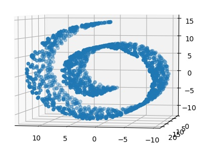
Assumes that the data lies in low-dimensional manifold (looks Euclidean in small neighborhoods)
Given dataset \(\calD=\{\bfx_i\}_{i=1}^N\in\bbR^d\), try to compute estimate of the geodesic distance along manifold
- How do we estimate the geodesic distance?
Estimating geodesic distance
Compute shortest path using a proximity graph
- Form a matrix \(\bfW\) as follows
- For every \(\bfx_i\) define local neighborhood \(\calN_i\) (e.g., \(k\) nearest neighbors, all \(\bfx_j\) s.t. \(\norm[2]{\bfx_j-\bfx_i}\leq \epsilon\))
- For each \(\bfx_i\), set \(w_{ij}=\norm[2]{\bfx_i-\bfx_j}\)
\(\bfW\) is a weighted adjacency matrix of the graph
Compute \(\bfD\) by setting \(d_{ij}\) to length of shortest path from node \(i\) to node \(j\) in graph described by \(\bfW\)
Can compute embedding similarly to MDS
Challenge: isomap can become inaccurate for points far apart
Locally linear embedding (LLE)
- Idea: a data manifold that is globally nonlinear still appears linear in local pieces
- Don’t try to explicitly model global geodesic distances
- Try to preserve structure in data by patching together local pieces of the manifold
- LLE algorithm for dataset \(\calD=\{\bfx_i\}_{i=1}^N\in\bbR^d\)
- For each \(\bfx_i\), define local neighborhood \(\calN_i\)
- Solve \[\min_\bfW \sum_{i=1}^N\norm[2]{\bfx_i-\sum_{j=1}^N w_{ij}\bfx_j}^2\text{ s.t. }\sum_{j}w_{ij}=1\text{ and }w_{ij}=0\text{ for }j\notin\calN_i\]
- Fix \(\bfW\) and solve \[\min_{\{\bftheta_i\}}\sum_{i=1}^N\norm[2]{\bftheta_i-\sum_{j=1}^Nw_{ij}\bftheta_j}^2\]
Locally linear embedding (LLE)
- Eigenvalue problem in compact form: \[\min_{\bfTheta}\norm[F]{\bfTheta-\bfTheta\bfW}^2=\min_{\bfTheta}\trace{\bfTheta(\bfI-\bfW)^\intercal(\bfI-\bfW)\bfTheta^\intercal}\]
- Same problem encountered in PCA!
- Use eigendecomposition of \((\bfI-\bfW)^\intercal(\bfI-\bfW)\)
- Can compute embedding of new points as \[\theta = \sum_{i=1}^N w_{\bfx,\bfx_i}\bftheta_i\] with \(w_{\bfx,\bfx_i}\) computed from same constrained least squares problem
Demo notebook