Bayes Classifiers
Matthieu R Bloch
Fundamental trade-off of learning
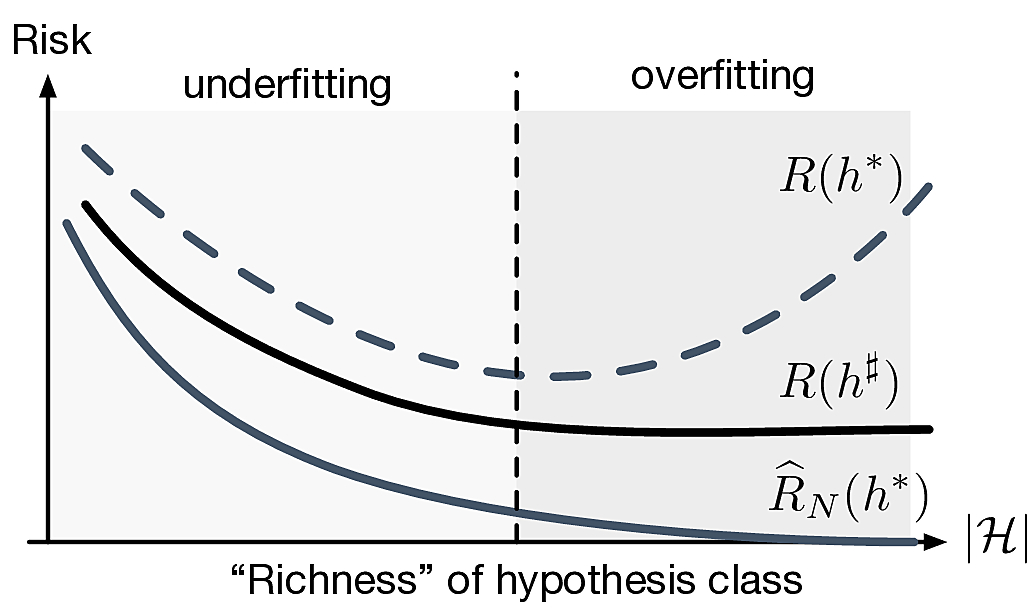
- Demo: generalization for nearest-neighbor classifier
Supervised learning model
We revisit the supervised learning setup (slight change in notation)
- Dataset \(\calD\eqdef\{(X_1,Y_1),\cdots,(X_N,Y_N)\}\)
- \(\{X_i\}_{i=1}^N\) drawn i.i.d. from unknown \(P_{X}\) on \(\calX=\bbR^d\)
- \(\{Y_i\}_{i=1}^N\) labels with \(\calY=\{0,1,\cdots,K-1\}\) (multiclass classification)
Unknown \(P_{Y|X}\)
Binary loss function \(\ell:\calY\times\calY\rightarrow\bbR^+:(y_1,y_2)\mapsto \indic{y_1\neq y_2}\)
The risk of a classifier \(h\) is \[ R(h)\eqdef\E[XY]{\indic{h(X)\neq Y}} = \P[X Y]{h(X)\neq Y} \]
We will not directly worry about \(\calH\), but rather about \(R(\hat{h}_N)\) for some \(\hat{h}_N\) that we will estimate from the data
Bayes classifier
- What is the best risk (smallest) that we can achieve?
- Assume that we actually know \(P_{X}\) and \(P_{Y|X}\)
- Denote the a posteriori class probabilities of \(\bfx\in\calX\) by \[ \eta_k(\bfx) \eqdef \P{Y=k|X=\bfx}\]
- Denote the a priori class probabilities by \[\pi_k\eqdef \P{Y=k}\]
The classifier \(h^\text{B}(\bfx)\eqdef\argmax_{k\in[0;K-1]} \eta_k(\bfx)\) is optimal, i.e., for any classifier \(h\), we have \(R(h^\text{B})\leq R(h)\). \[ R(h^{\text{B}}) = \E[X]{1-\max_k \eta_k(X)} \]
- Terminology
- \(h^B\) is called the Bayes classifier
- \(R_B\eqdef R(h^B)\) is called the Bayes risk
Other forms of the Bayes classifier
\(h^\text{B}(\bfx)\eqdef\argmax_{k\in[0;K-1]} \eta_k(\bfx)\)
\(h^\text{B}(\bfx)\eqdef\argmax_{k\in[0;K-1]} \pi_k p_{X|Y}(\bfx|k)\)
For \(K=2\) (binary classification): log-likelihood ratio test \[ \log\frac{p_{X|Y}(\bfx|1)}{p_{X|Y}(\bfx|0)} \gtrless \log \frac{\pi_0}{\pi_1} \]
If all classes are equally likely \(\pi_0=\pi_1=\cdots=\pi_{K-1}\) \[ h^\text{B}(\bfx)\eqdef\argmax_{k\in[0;K-1]} p_{X|Y}(\bfx|k) \]
Assume \(X|Y=0\sim\calN(0,1)\) and \(X|Y=1\sim\calN(1,1)\). The Bayes risk for \(\pi_0=\pi_1\) is \(R(h^\text{B})=\Phi(-\frac{1}{2})\) with \(\Phi\eqdef\text{Normal CDF}\)
- In practice we do not know \(P_X\) and \(P_{Y|X}\)
- Plugin methods: use the data to learn the distributions and plug result in Bayes classifier
Other loss functions
We have focused on the risk \(\P{h(X)\neq Y}\) obtained for a binary loss function \(\indic{h(X)\neq Y}\)
- There are many situations in which this is not appropriate
- Cost sensitive classification: false alarm and missed detection may not be equivalent \[ c_0\indic{h(X)\neq 0\text{ and }Y=0} + c_1 \indic{h(X)\neq 1\text{ and }Y=1} \]
- Unbalanced data set: the probability of the largest class will dominate