Learning

Logistics

• General announcements

  • Assignment 6 due December 7, 2021 for bonus, deadline December 10, 2021

  • Last lecture!

  • Let me know what’s missing

  • Expect an email from me tonight

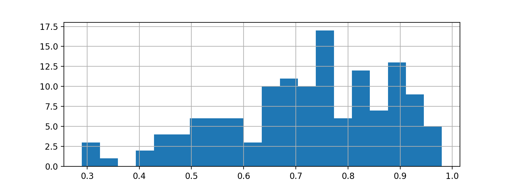
• Midterm 2 statistics

  • Overall: AVG: 72% - MIN: 29% - MAX: 98%

What we have learned this Fall

• Hilbert spaces

  • Spaces of functions can be manipulated almost just as easily

  • Finite dimensional is fairly natural

  • Infinite dimensional can be manipulated just as well using orthobases

  • With orthobases, vectors in infinite dimensional separates Hilbert spaces are like square summable sequences

• Regression

  • Who knew solving \(\vecy=\matA\vecx\) could be so useful?

  • SVD provides lots of insights

• Regression in Hilbert spaces

  • Perhaps biggest lesson of the course
  • Representer theorem allows us to do regression in infinite dimensional Hilbert spaces
  • RKHS provide the kind of Hilbert spaces that naturally embed our data

What’s on the agenda for today?

• More on learning and Bayes classifiers

• Lecture notes 17 and 23

A simpler supervised learning problem

Consider a special case of the general supervised learning problem

1. Dataset \(\calD\eqdef\{(\bfx_1,y_1),\cdots,(\bfx_N,y_N)\}\)

   • \(\{\bfx_i\}_{i=1}^N\) drawn i.i.d. from unknown \(P_{\bfx}\) on \(\calX\)
   • \(\{y_i\}_{i=1}^N\) labels with \(\calY=\{0,1\}\) (binary classification)

2. Unknown \(f:\calX\to\calY\), no noise.

3. Finite set of hypotheses \(\calH\), \(\card{\calH}=M<\infty\)

   • \(\calH\eqdef\{h_i\}_{i=1}^M\)

4. Binary loss function \(\ell:\calY\times\calY\rightarrow\bbR^+:(y_1,y_2)\mapsto \indic{y_1\neq y_2}\)

• In this very specific case, the true risk simplifies \[ R(h)\eqdef\E[\bfx y]{\indic{h(\bfx)\neq y}} = \P[\bfx y]{h(\bfx)\neq y} \]

• The empirical risk becomes \[ \widehat{R}_N(h)=\frac{1}{N}\sum_{i=1}^{N} \indic{h(\bfx_i)\neq y_i} \]

Can we learn?

• Our objective is to find a hypothesis \(h^*=\argmin_{h\in\calH}\widehat{R}_N(h)\) that ensures a small risk

• For a fixed \(h_j\in\calH\), how does \(\widehat{R}_N(h_j)\) compares to \({R}(h_j)\)?

• Observe that for \(h_j\in\calH\)

  • The empirical risk is a sum of iid random variables \[ \widehat{R}_N(h_j)=\frac{1}{N}\sum_{i=1}^{N} \indic{h_j(\bfx_i)\neq y_i} \]

  • \(\E{\widehat{R}_N(h_j)} = R(h_j)\)

• \(\P{\abs{\widehat{R}_N(h_j)-{R}(h_j)}>\epsilon}\) is a statement about the deviation of a normalized sum of iid random variables from its mean

• We’re in luck! Such bounds, a.k.a, known as concentration inequalities, are a well studied subject

Concentration inequalities: basics

• Let \(X\) be a non-negative real-valued random variable. Then for all \(t>0\) \[\P{X\geq t}\leq \frac{\E{X}}{t}.\]

• Let \(X\) be a real-valued random variable. Then for all \(t>0\) \[\P{\abs{X-\E{X}}\geq t}\leq \frac{\Var{X}}{t^2}.\]

• Let \(\{X_i\}_{i=1}^N\) be i.i.d. real-valued random variables with finite mean \(\mu\) and finite variance \(\sigma^2\). Then \[\P{\abs{\frac{1}{N}\sum_{i=1}^N X_i-\mu}\geq\epsilon}\leq\frac{\sigma^2}{N\epsilon^2}\qquad\lim_{N\to\infty}\P{\abs{\frac{1}{N}\sum_{i=1}^N X_i-\mu}\geq \epsilon}=0.\]

Back to learning

• By the law of large number, we know that \[ \forall\epsilon>0\quad\P[\{(\bfx_i,y_i)\}]{\abs{\widehat{R}_N(h_j)-{R}(h_j)}\geq\epsilon}\leq \frac{\Var{\indic{h_j(\bfx_1)\neq y_1}}}{N\epsilon^2}\leq \frac{1}{N\epsilon^2}\]

• Given enough data, we can generalize

• How much data? \(N=\frac{1}{\delta\epsilon^2}\) to ensure \(\P{\abs{\widehat{R}_N(h_j)-{R}(h_j)}\geq\epsilon}\leq \delta\).

• That’s not quite enough! We care about \(\widehat{R}_N(h^*)\) where \(h^*=\argmin_{h\in\calH}\widehat{R}_N(h)\)

  • If \(M=\card{\calH}\) is large we should expect the existence of \(h_k\in\calH\) such that \(\widehat{R}_N(h_k)\ll R(h_k)\)

• \[ \P{\abs{\widehat{R}_N(h^*)-{R}(h^*)}\geq\epsilon} \leq \P{\exists j:\abs{\widehat{R}_N(h_j)-{R}(h_j)}\geq\epsilon} \]

• \[ \P{\abs{\widehat{R}_N(h^*)-{R}(h^*)}\geq\epsilon} \leq \frac{M}{N\epsilon^2} \]

• If we choose \(N\geq\lceil\frac{M}{\delta\epsilon^2}\rceil\) we can ensure \(\P{\abs{\widehat{R}_N(h^*)-{R}(h^*)}\geq\epsilon}\leq \delta\).

  • That’s a lot of samples!

Concentration inequalities: not so basic

• We can obtain much better bounds than with Chebyshev

• Let \(\{X_i\}_{i=1}^N\) be i.i.d. real-valued zero-mean random variables such that \(X_i\in[a_i;b_i]\) with \(a_i<b_i\). Then for all \(\epsilon>0\) \[\P{\abs{\frac{1}{N}\sum_{i=1}^N X_i}\geq\epsilon}\leq 2\exp\left(-\frac{2N^2\epsilon^2}{\sum_{i=1}^N(b_i-a_i)^2}\right).\]

• In our learning problem \[ \forall\epsilon>0\quad\P{\abs{\widehat{R}_N(h_j)-{R}(h_j)}\geq\epsilon}\leq 2\exp(-2N\epsilon^2)\]

• \[ \forall\epsilon>0\quad\P{\abs{\widehat{R}_N(h^*)-{R}(h^*)}\geq\epsilon}\leq 2M\exp(-2N\epsilon^2)\]

• We can now choose \(N\geq \lceil\frac{1}{2\epsilon^2}\left(\ln \frac{2M}{\delta}\right)\rceil\)

• \(M\) can be quite large (almost exponential in \(N\)) and, with enough data, we can generalize \(h^*\).

• How about learning \(h^{\sharp}\eqdef\argmin_{h\in\calH}R(h)\)?

Learning can work!

• If \(\forall j\in\calH\,\abs{\widehat{R}_N(h_j)-{R}(h_j)}\leq\epsilon\) then \(\abs{R(h^*)-{R}(h^\sharp)}\leq 2\epsilon\).

• How do we make \(R(h^\sharp)\) small?

  • Need bigger hypothesis class \(\calH\)! (could we take \(M\to\infty\)?)
  • Fundamental trade-off of learning

Probably Approximately Correct Learnability

• A hypothesis set \(\calH\) is (agnostic) PAC learnable if there exists a function \(N_\calH:]0;1[^2\to\bbN\) and a learning algorithm such that:

  • for very \(\epsilon,\delta\in]0;1[\),
  • for every \(P_\bfx\), \(P_{y|\bfx}\),
  • when running the algorithm on at least \(N_\calH(\epsilon,\delta)\) i.i.d. examples, the algorithm returns a hypothesis \(h\in\calH\) such that \[\P[\bfx y]{\abs{{R}(h)-R(h^\sharp)}\leq\epsilon}\geq 1-\delta\]

• The function \(N_{\calH}(\epsilon,\delta)\) is called sample complexity

• We have effectively already proved the following result

• A finite hypothesis set \(\calH\) is PAC learnable with the Empirical Risk Minimization algorithm and with sample complexity \[N_\calH(\epsilon,\delta)={\lceil{\frac{2\ln(2\card{\calH}/\delta)}{\epsilon^2}}\rceil}\]

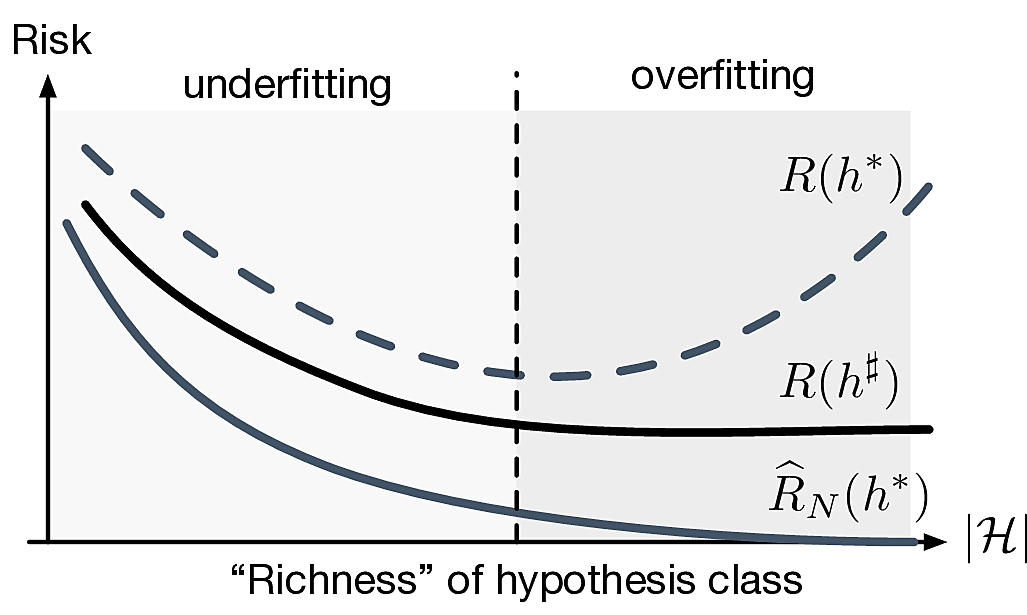
What is a good hypothesis set?

• Ideally we want \(\card{\calH}\) small so that \(R(h^*)\approx R(h^\sharp)\) and get lucky so that \(R(h^*)\approx 0\)

• In general this is not possible

• Remember, we usually have to learn \(P_{y|\bfx}\), not a function \(f\)

• Questions

  • What is the optimal binary classification hypothesis class?
  • How small can \(R(h^*)\) be?

Supervised learning model

We revisit the supervised learning setup (slight change in notation)

1. Dataset \(\calD\eqdef\{(X_1,Y_1),\cdots,(X_N,Y_N)\}\)

   • \(\{X_i\}_{i=1}^N\) drawn i.i.d. from unknown \(P_{X}\) on \(\calX=\bbR^d\)
   • \(\{Y_i\}_{i=1}^N\) labels with \(\calY=\{0,1,\cdots,K-1\}\) (multiclass classification)

2. Unknown \(P_{Y|X}\)

3. Binary loss function \(\ell:\calY\times\calY\rightarrow\bbR^+:(y_1,y_2)\mapsto \indic{y_1\neq y_2}\)

• The risk of a classifier \(h\) is \[ R(h)\eqdef\E[XY]{\indic{h(X)\neq Y}} = \P[X Y]{h(X)\neq Y} \]

• We will not directly worry about \(\calH\), but rather about \(R(\hat{h}_N)\) for some \(\hat{h}_N\) that we will estimate from the data

Bayes classifier

• What is the best risk (smallest) that we can achieve?
  • Assume that we actually know \(P_{X}\) and \(P_{Y|X}\)
  • Denote the a posteriori class probabilities of \(\bfx\in\calX\) by \[ \eta_k(\bfx) \eqdef \P{Y=k|X=\bfx}\]
  • Denote the a priori class probabilities by \[\pi_k\eqdef \P{Y=k}\]

• The classifier \(h^\text{B}(\bfx)\eqdef\argmax_{k\in[0;K-1]} \eta_k(\bfx)\) is optimal, i.e., for any classifier \(h\), we have \(R(h^\text{B})\leq R(h)\). \[ R(h^{\text{B}}) = \E[X]{1-\max_k \eta_k(X)} \]

• Terminology
  • \(h^B\) is called the Bayes classifier
  • \(R_B\eqdef R(h^B)\) is called the Bayes risk

Other forms of the Bayes classifier

• \(h^\text{B}(\bfx)\eqdef\argmax_{k\in[0;K-1]} \eta_k(\bfx)\)

• \(h^\text{B}(\bfx)\eqdef\argmax_{k\in[0;K-1]} \pi_k p_{X|Y}(\bfx|k)\)

• For \(K=2\) (binary classification): log-likelihood ratio test \[ \log\frac{p_{X|Y}(\bfx|1)}{p_{X|Y}(\bfx|0)} \gtrless \log \frac{\pi_0}{\pi_1} \]

• If all classes are equally likely \(\pi_0=\pi_1=\cdots=\pi_{K-1}\) \[ h^\text{B}(\bfx)\eqdef\argmax_{k\in[0;K-1]} p_{X|Y}(\bfx|k) \]

• Assume \(X|Y=0\sim\calN(0,1)\) and \(X|Y=1\sim\calN(1,1)\). The Bayes risk for \(\pi_0=\pi_1\) is \(R(h^\text{B})=\Phi(-\frac{1}{2})\) with \(\Phi\eqdef\text{Normal CDF}\)

• In practice we do not know \(P_X\) and \(P_{Y|X}\)

  • Plugin methods: use the data to learn the distributions and plug result in Bayes classifier

Nearest neighbor classifier

• Back to our training dataset \(\calD\eqdef\{(\bfx_1,y_1),\cdots,(\bfx_N,y_N)\}\)

• The nearest-neighbor (NN) classifier is \(h^{\text{NN}}(\bfx)\eqdef y_{\text{NN}(\bfx)}\) where \(\text{NN}(\bfx)\eqdef \argmin_i \norm{\bfx_i-\bfx}\)

• Risk of NN classifier conditioned on \(\bfx\) and \(\bfx_{\text{NN}(\bfx)}\) \[ R_{\text{NN}}(\bfx,\bfx_{\text{NN}(\bfx)}) = \sum_{k}\eta_k(\bfx_{\text{NN}(\bfx)})(1-\eta_k(\bfx))= \sum_{k}\eta_k(\bfx)(1-\eta_k(\bfx_{\text{NN}(\bfx)})). \]

  • How well does the average risk \(R_{\text{NN}}=R(h^{\text{NN}})\) compare to the Bayes risk for large \(N\)?

• Let \(\bfx\), \(\{\bfx_i\}_{i=1}^N\) be i.i.d. \(\sim P_{\bfx}\) in a separable metric space \(\calX\). Let \(\bfx_{\text{NN}(\bfx)}\) be the nearest neighbor of \(\bfx\). Then \(\bfx_{\text{NN}(\bfx)} \to \bfx\) with probability one as \(N\to\infty\)

• Let \(\calX\) be a separable metric space. Let \(p(\bfx|y=0)\), \(p(\bfx|y=1)\) be such that, with probability one, \(\bfx\) is either a continuity point of \(p(\bfx|y=0)\) and \(p(\bfx|y=1)\) or a point of non-zero probability measure. As \(N\to\infty\), \[R(h^{\text{B}}) \leq R(h^{\text{NN}})\leq 2R(h^{\text{B}})(1-R(h^{\text{B}}))\]

K Nearest neighbors classifier

• Can drive the risk of the NN classifier to the Bayes risk by increasing the size of the neighborhood
  • Assign label to \(\bfx\) by taking majority vote among \(K\) nearest neighbors \(h^\text{$K$-NN}\) \[\lim_{N\to\infty}\E{R(h^{\text{$K$-NN}})}\leq \left(1+\sqrt{\frac{2}{K}}\right)R(h^{\text{B}})\]

• Let \(\hat{h}_N\) be a classifier learned from \(N\) data points; \(\hat{h}_N\) is consistent if \(\E{R(\hat{h}_N)}\to R_B\) as \(N\to\infty\).

• If \(N\to\infty\), \(K\to\infty\), \(K/N\to 0\), then \(h^{\text{$K$-NN}}\) is consistent

• Choosing \(K\) is a problem of model selection
  • Do not choose \(K\) by minimizing the empirical risk on training: \[\widehat{R}_N(h^{\text{$1$-NN}}) = \frac{1}{N}\sum_{i=1}^N\indic{h_1(\bfx_i)=y_i}=0\]
  • Need to rely on estimates from model selection techniques (more later!)