Mathematical Foundations of Machine Learning

Prof. Matthieu Bloch

Monday, October 28, 2024

Last time

Last class: Wednesday October 23, 2024
- We proved about the spectral theorem
- We talked about relating the spectral theorem to the stability of solutions of \(\vecy=\matA\vecx\)
  - (\(\matA\) square and postive definite)
Today: We will talk about the singular value decomposition

To be effectively prepared for today's class, you should have:
1. Gone over slides and read associated lecture notes here
2. Started working on Homework 5 (due Tuesday October 29, 2024)
Logistics: use office hours to prepare for Homework 5
- Jack Hill office hours: Wednesday 11:30am-12:30pm in TSRB and hybrid
- Anuvab Sen office hours: Thursday 12pm-1pm in TSRB and hybrid
Homework 6: due Thursday November 7, 2024

Wednesday October 30, 2024 no synchronous class
- I am traveling to a conference and will upload an asynchronous lecture

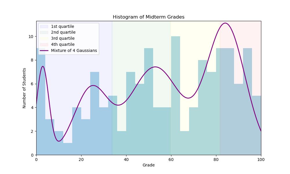
Midterm statistics

What can we do

We will be introducing recitations with GTAs every week
- Opportunity to go through examples
- Opportunity to work on a problem with some guidance
Think about your study habits

Spectral theorem

Every complex matrix \(\matA\) has at least one complex eigenvector and every real symmetrix matrix has real eigenvalues and at least one real eigenvector.

Every matrix \(\matA\in\bbC^{n\times n}\) is unitarily similar to an upper triangular matrix, i.e., \[ \bfA = \bfV\boldsymbol{\Delta}\bfV^\dagger \] with \(\boldsymbol{\Delta}\) upper triangular and \(\bfV^\dagger=\bfV^{-1}\).

Every hermitian matrix is unitarily similar to a real-valued diagonal matrix.

Note that if \(\matA = \matV\matD\matV^\dagger\) then \(\matA = \sum_{i=1}^n\lambda_i \vecv_i\vecv_i^\dagger\)

How about real-valued matrices \(\matA\in\bbR^{n\times n}\)?

Singular value decomposition

What happens for non-square matrices?

Let \(\matA\in\bbR^{m\times n}\) with \(\text{rank}(\matA)=r\). Then \(\matA=\matU\boldsymbol{\Sigma}\matV^T\) where

\(\matU\in\bbR^{m\times r}\) such that \(\matU^\intercal\matU=\bfI_r\) (orthonormal columns)
\(\matV\in\bbR^{n\times r}\) such that \(\matV^\intercal\matV=\bfI_r\) (orthonormal columns)
\(\boldsymbol{\Sigma}\in\bbR^{r\times r}\) is diagonal with positive entries

\[ \boldsymbol{\Sigma}\eqdef\mat{cccc}{\sigma_1&0&0&\cdots\\0&\sigma_2&0&\cdots\\\vdots&&\ddots&\\0&\cdots&\cdots&\sigma_r} \] and \(\sigma_1\geq\sigma_2\geq\cdots\geq\sigma_r>0\). The \(\sigma_i\) are called the singular values

We say that \(\matA\) is full rank is \(r=\min(m,n)\)
We can write \(\matA=\sum_{i=1}^r\sigma_i\vecu_i\vecv_i^\intercal\)

Important properties of the SVD

The columns of \(\matV\) \(\set{\vecv_i}_{i=1}^r\) are eigenvectors of the psd matrix \(\matA^\intercal\matA\).
- \(\set{\sigma_i:1\leq i\leq n\text{ and } \sigma_i\neq 0}\) are the square roots of the non-zero eigenvalues of \(\matA^\intercal\matA\).
The columns of \(\matU\) \(\set{\vecu_i}_{i=1}^r\) are eigenvectors of the psd matrix \(\matA\matA^\intercal\).
- \(\set{\sigma_i:1\leq i\leq n\text{ and } \sigma_i\neq 0}\) are the square roots of the non-zero eigenvalues of \(\matA\matA^\intercal\).
The columns of \(\matV\) form an orthobasis for \(\text{row}(\matA)\)

The columns of \(\matU\) form an orthobasis for \(\text{col}(\matA)\)

Equivalent form of the SVD: \(\matA=\widetilde{\matU}\widetilde{\boldsymbol{\Sigma}}\widetilde{\matV}^T\) where
- \(\widetilde{\matU}\in\bbR^{m\times m}\) is orthonormal
- \(\widetilde{\matV}\in\bbR^{n\times n}\) is orthonormal
- \(\widetilde{\boldsymbol{\Sigma}}\in\bbR^{m\times n}\) is
\[ \widetilde{\boldsymbol{\Sigma}}\eqdef\mat{cc}{\boldsymbol{\Sigma}&\boldsymbol{0}\\\boldsymbol{0}&\boldsymbol{0}} \]

SVD and least-squares

When we cannot solve \(\vecy=\matA\vecx\), we solve instead \[ \min_{\bfx\in\bbR^n}\norm[2]{\vecx}^2\text{ such that } \matA^\intercal\matA\vecx = \matA^\intercal\vecy \]
- This allows us to pick the minimum norm solution among potentially infinitely many solutions of the normal equations.
Recall: when \(\matA\in\bbR^{m\times n}\) is of rank \(m\), then \(\bfx=\matA^\intercal(\matA\matA^\intercal)^{-1}\vecy\)

The solution of \[ \min_{\bfx\in\bbR^n}\norm[2]{\vecx}^2\text{ such that } \matA^\intercal\matA\vecx = \matA^\intercal\vecy \] is \[ \hat{\vecx} = \matV\boldsymbol{\Sigma}^{-1}\matU^\intercal\vecy = \sum_{i=1}^r\frac{1}{\sigma_i}\dotp{\vecy}{\vecu_i}\vecv_i \] where \(\matA=\matU\boldsymbol{\Sigma}\matV^T\) is the SVD of \(\matA\).

Pseudo inverse

\(\matA^+ = \matV\boldsymbol{\Sigma}^{-1}\matU^\intercal\) is called the pseudo-inverse, Lanczos inverse, or Moore-Penrose inverse of \(\matA=\matU\boldsymbol{\Sigma}\matV^T\).

If \(\matA\) is square invertible then \(\matA^+=\matA\)

If \(m\geq n\) (tall and skinny matrix) of rank \(n\) then \(\matA^+ = (\matA^\intercal\matA)^{-1}\matA^\intercal\)

If \(m\geq n\) (short and fat matrix) of rank \(m\) then \(\matA^+ = \matA^\intercal(\matA\matA^\intercal)^{-1}\)

Note \(\matA^+\) is as "close" to an inverse of \(\matA\) as possible

Stability of least squares

What if we observe \(\vecy = \matA\vecx_0+\vece\) and we apply the pseudo inverse? \(\hat{\vecx} = \matA^+\vecy\)

We can separate the error analysis into two components \[ \hat{\vecx}-\vecx_0 = \underbrace{\matA^+\matA\vecx_0-\vecx_0}_{\text{null space error}} + \underbrace{\matA^+\vece}_{\text{noise error}} \]
We will express the error in terms of the SVD \(\matA=\matU\boldsymbol{\Sigma}\matV^\intercal\) With
- \(\set{\vecv_i}_{i=1}^r\) orthobasis of \(\text{row}(\matA)\), augmented by \(\set{\vecv_i}_{i=1}^{r+1}\in\ker{\matA}\) to form an orthobasis of \(\bbR^n\)
- \(\set{\vecu_i}_{i=1}^r\) orthobasis of \(\text{col}(\matA)\), augmented by \(\set{\vecu}_{i=1}^{r+1}\in\ker{\matA^\intercal}\) to form an orthobasis of \(\bbR^m\)
The null space error is given by \[ \norm[2]{\matA^+\matA\vecx_0-\vecx_0}^2=\sum_{i=r+1}^n\abs{\dotp{\vecv_i}{x_0}}^2 \]
The noise error is given by \[ \norm[2]{\matA^+\vece}^2=\sum_{i=1}^r \frac{1}{\sigma_i^2}\abs{\dotp{\vece}{\vecu_i}}^2 \]

Stable reconstruction by truncation

How do we mitigate the effect of small singular values in reconstruction? \[ \hat{\vecx} = \matV\boldsymbol{\Sigma}^{-1}\matU^\intercal\vecy = \sum_{i=1}^r\frac{1}{\sigma_i}\dotp{\vecy}{\vecu_i}\vecv_i \]
Truncate the SVD to \(r'<r\) \[ \matA_t\eqdef \sum_{i=1}^{r'}\sigma_i\vecu_i\vecv_i^\intercal\qquad\matA_t^+ = \sum_{i=1}^{r'}\frac{1}{\sigma_i}\vecu_i\vecv_i^\intercal \]
Reconstruct \(\hat{\vecx_t} = \sum_{i=1}^{r'}\frac{1}{\sigma_i}\dotp{\vecy}{\vecu_i}\vecv_i=\matA_t\)

Error analysis: \[ \norm[2]{\hat{\vecx}_t-\vecx_0}^2 = \sum_{i=r+1}^n\abs{\dotp{\vecx_0}{\vecv_i}}^2+\sum_{i=r'+1}^r\abs{\dotp{\vecx_0}{\vecv_i}}^2+\sum_{i=1}^r'\frac{1}{\sigma_i^2}\abs{\dotp{\vece}{\vecu_i}}^2 \]

Stable reconstruction by regularization

Regularization means changing the problem to solve \[ \min_{\vecx\in\bbR^n}\norm[2]{\vecy-\matA\vecx}^2+\lambda\norm[2]{\vecx}^2\qquad\ \lambda>0 \]
The solution is \[ \hat{\vecx} = (\matA^\intercal\matA+\lambda\matI)^{-1}\matA^\intercal\vecy = \matV(\boldsymbol{\Sigma}^2+\lambda\matI)^{-1}\boldsymbol{\Sigma}\matU^\intercal\vecy \]

Numerical methods

We have seen several solutions to systems of linear equations \(\matA\vecx=\vecy\) so far
- \(\matA\) full column rank: \(\hat{\bfx} = (\matA^\intercal\matA)^{-1}\matA^\intercal\bfy\)
- \(\matA\) full row rank: \(\hat{\bfx} = \matA^\intercal(\matA\matA^\intercal)^{-1}\bfy\)
- Ridge regression: \(\hat{\bfx} = (\matA^\intercal\matA+\delta\matI)^{-1}\matA^\intercal\bfy\)
- Kernel regression: \(\hat{\bfx} = (\matK+\delta\matI)^{-1}\bfy\)
- Ridge regression in Hilbert space: \(\hat{\bfx} = (\matA^\intercal\matA+\delta\matG)^{-1}\matA^\intercal\bfy\)
Extension: constrained least-squares \[ \min_{\vecx\in\bbR^n}\norm[2]{\vecy-\matA\vecx}^2\text{ s.t. } \vecx=\matB\vecalpha\text{ for some }\vecalpha \]
- The solution is \(\hat{\bfx} = \matB(\matB^\intercal\matA^\intercal\matA\matB)^{-1}\matB^\intercal\matA^\intercal\bfy\)
All these problems involve a symmetric positive definite system of equations.
- Many methods to achieve this based on matrix factorization

Next time

Next class: Wednesday October 30, 2024 (asynchronous)

To be effectively prepared for next class, you should:
1. Go over today's slides and read associated lecture notes
2. Work on Homework 5
Optional
- Export slides for next lecture as PDF (be on the lookout for an announcement when they're ready)